Summary

Nucleus motorized microscopes from Zaber form a compact benchtop microscope platform that offers a flexible configuration to adapt the user needs, and includes fast and precise motorized XY and Z-focus movement devices. Nucleus microscopes are fully controlled by the Inscoper I.S. control and image acquisition solution, allowing users to benefit from its combination with a complete and easy-to-use imaging software.

We show in this technical note how fast is the Zaber X-ADR XY stage of the Nucleus microscope compared to a regular one.

ZABER PRODUCTS

Zaber (Vancouver, BC, Canada) designs and manufactures positioning devices such as linear or rotational stages, optical mounts, micromanipulators, stepper motors which are used in different industries, including microscopy and life science.

Zaber products also include the Nucleus modular automated microscope platform which includes both upright and inverted microscopes. They are designed to be compact, customized and affordable.

In this note we focus on the Nucleus platform but it is worth noting that all devices from Zaber can be easily integrated in the I.S. solution thanks to convenient software tools (device library, communication protocols).

NUCLEUS motorized microscope for 5D fluorescence imaging

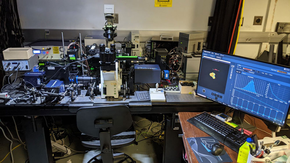
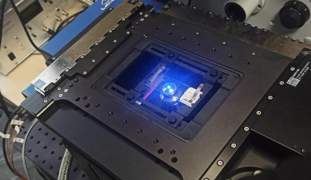
Zaber Nucleus microscopes are compact (Figure 1), and suitable to be used in a laboratory environment or a microscopy imaging core facility. They include a motorized XY stage and a motorized Z-focus, white light for bright field illumination, three LED illumination sources and 6 filter positions for fluorescence imaging. Up to two C-mount camera ports are available, for maximum compatibility with cameras available on the market. The objective holders are compatible with optics from all four manufacturers (Evident, Leica, Nikon, Zeiss).

Nucleus microscope have a flexible configuration: they can be adapted or customized to user needs and applications such as BrightField, Epifluorescence or multi-well plate screening.

Figure 1: Zaber Nucleus inverted microscope

Integration and performance tests with Inscoper I.S.

INSCOPER (Cesson-Sévigné, France) develops software solutions for device control and image acquisition in microscopy. Its main product I.S. is compatible with all camera-based microscope setups and dedicated to a large panel of applications such as live cell imaging, confocal imaging, ratiometric imaging, light-sheet microscopy, super-resolution, photomanipulation (FRAP) or FLIM imaging.

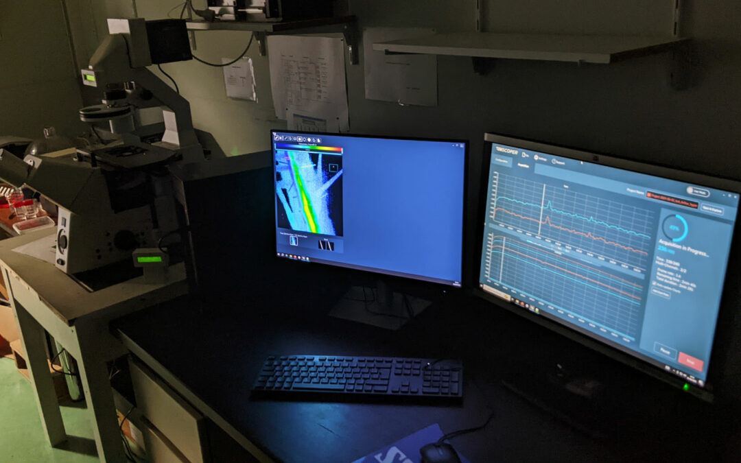
I.S. offers a user-friendly graphical user interface (Figure 2) allowing the full control and combination of all motorized devices, multidimensional acquisitions (time, XYZ, channels, multi-positions, tiling) and image visualization. It consists of one window with three tabs (Configuration, Acquisition, Visualization) and has been designed to address all kinds of needs in microscopy acquisition with the aim to always keep a simple and intuitive user exprience.

Figure 2: user-friendly interface, Acquisition tab with multidimensional acquisition model

You can watch on this demo video how easy it is to navigate in the I.S. software environment to configure and acquire images with a Zaber Nucleus microscope.

Test conditions

A special feature of the I.S imaging solution is that it is based on a technology that eliminates all software latency when communicating with the microscope devices to control. This feature allows users to benefit from 2x to 4x higher frame rate for their acquisitions. But it is also particularly useful when testing motorized devices such as stages, because we are certain to compare their strict hardware performance with no impact or variation caused by software drivers or the computer’s operating system.

Another essential feature for technical analysis is that I.S. generates a “performance file” associated with each acquisition. The duration of each command for each device is recorded down to the microsecond, enabling a very detailed and precise study of acquisition performance.

For this technical note we performed two sets of tests:

• We compared the performance of a Zaber Nucleus X-ADR stage with a standard stage (Nikon Ti2) in acquiring a tiled imaging,
• We simulated maximum stages performance for moving from one point to another randomly in X and Y directions.

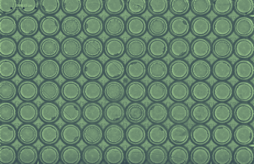
Figure 3: Tiling imaging of Mouse kidney (60 tiles) acquired with a Nucleus microscope (Zaber) using a Zeiss 20x objective. The same acquisition was performed with a standard microscope (Nikon Ti2). Label is WGA 488 nm, GFP filter has 466/48 nm excitation and 525/49nm emission.

XY scanning speed when acquiring a tiled image

In this first set of tests, we performed a tile imaging experiment of mouse kidney with a 20x objective (Figure 3). The acquisition sequence was exactly the same for each microscope, Zaber Nucleus and Ti2: 60 tiles with 10 rows and 6 columns set in fastest “snake” mode (first row acquired from left to right, then second row from right to left, etc.). Exposure time was 30 milliseconds.

Thanks to the performance file, the precise scanning speed for the tiling acquisition for each system is recorded for each movement at the microsecond. Results are shown in Table I: the average XY scanning speed, including the exposure time, was 4.3 mm²/s for the MVR and 1.2 mm²/s for the Ti2. The XY scanning speed of the Nucleus microscope was 3.5 times faster in average than the Ti2 for this tile imaging experiment. This XY “surface” speed does not discriminate between the X and Y axis, what we will do next.

Table I: Scanning speed comparison between Zaber Nucleus and Nikon Ti2 microscopes for the same image acquisition sequence

Maximum XY scanning speed

In this second set of tests, we compared the time taken to move each stage from one position to another as quickly as possible.

To ensure greater measurement reliability and equal test conditions between the two stages, we used an internal software tool that generates random X,Y coordinates within a defined maximum range. Ninety-nine (99) random positions were generated within a motion range of 0 to 25 mm.

The maximum speed of the standard stage tends towards 21 mm/s for X and Y axes, which corresponds to Nikon specifications (approx. 25 mm/s).

The maximum speed of the Zaber X-ADR stage reaches 160 mm/s in the Y axis and 100 mm/s in the X axis at the longest travel distance tested, with no clear convergence to a maximum value.

We know from Zaber that the difference between both axes is due to the additional mass of the lower axis (X), and that the default maximum speed for this stage is 250 mm/s. This value could be reached with longer distances than those performed in this test. It can be increased up to 750 mm/s, but Zaber warns that it will also increase the acceleration (dv/dt) which may be problematic for the well being of some samples, and can also generate some vibrations that would increase the settling time.

Figure 4: Comparison of X-axis and Y-axis movement speed between Zaber and Nikon stages as a function of distance traveled

Then, we extracted the polynomial function of each speed curve from the Figure 4 to calculate the theoretical ratio between the two systems (Zaber/Nikon) and for each axis.

Results are shown in Figure 5. We note the systematic and significant outperformance of the Zaber stage compared to the reference stage, whatever the distance to be covered.

Both curves have a minimum around 2 to 2.5 mm travel distance, corresponding to an outperformance factor of 3x for the X axis and 5x for the Y axis. Depending on the distance, the Zaber stage moves at least 3 times faster on the X axis, with a maximum of 5 times at 25 mm, and at least 5 times faster on the Y axis, with a maximum of 9.8 times for 0.25 mm.

We found no positioning problems or precision errors during our tests. Please remember that these values were obtained using the I.S. imaging solution which adds no software latency to the hardware time required for movement.

Figure 5: Ratio as a function of the distance traveled between the speed of Zaber and Nikon stages for each axis (X in red, Y on green)

Fluorescence phenomenon in microscopy can be characterized by its intensity, but also by the time between the excitation of a fluorescent molecule and the emission of the corresponding photon. This measure of time is a microscopy technique called FLIM, for “Fluorescence Lifetime Imaging Microscopy’’. Here, we present a new opportunity for biological researchers to equip their microscope with the combination of the specialized pco.flim camera from Excelitas PCO (Germany) and the  Imaging Solution,  for microscope automation and image acquisition workflow from INSCOPER (France).

FLUORESCENCE-LIFETIME IMAGING FOR LIFE SCIENCE

Fluorescence is nowadays one of the most widely used techniques for the identification and localization of proteins in cells when coupled with specific antibodies or fused with proteins of interest (Moore & Morse, 1988; Lin et al, 2015). It is a phenomenon that consists of the absorption of light (ultraviolet or visible light), followed by the emission of photons with lower energy. Briefly, when a molecule (chemicals, protein, …) is excited at the appropriate wavelength, electrons change from a ground state to an excited state. When the molecule returns to the ground state, energy is released with photons emissions at a different longer wavelength of lower energy (Lakowicz, 2006).

Characterization of fluorescence signals can be done using its intensity, but also measuring its lifetime (time that a molecule stays in the excited state (S₁) before going back to the ground state (S₀) after excitation) or decay time (fluorescence decay curve after excitation). These measurements are performed using FLIM, for “Fluorescence-lifetime imaging microscopy”. Lifetime imaging allows the visualization and analysis of different structures and/or metabolic processes. One of the main applications of FLIM is to measure the Förster Resonance Energy Transfer (FRET), which allows to evaluate the proximity between two labeled-molecules or to monitor fluorescent biosensors.

There are two technical approaches (Figure 1) to measure fluorescence lifetimes, each with advantages and disadvantages.

Figure 1: Time- and frequency-domain measurements for FLIM
A representative overview of excitation (blue) and emission (turquoise) signals in time- and frequency-domain FLIM. (A) For the time-domain approach, excitation is performed using a pulsed laser and the fluorescence decay is directly measured. The fluorescence lifetime is measured by fitting the fluorescence decay. (B) For the frequency-domain, the excitation laser is continuously modulated and the emission signal is recovered. Some parameters including the amplitude (a_exc and a_em), the constant and direct components (b_exc and b_em) and the phase shift (Φ) are then used to determine the fluorescence lifetime.

1. The time-domain FLIM method consists of acquiring the decay curve of fluorescence (Delbarre et al, 2006). The most commonly used method is the TCSPC (Time Correlated Single Photon Counting). Using a pulsed laser, it can detect photons individually and reconstruct a decay curve to determine the exact fluorescence lifetime. This technique is suitable with mixed signals (multiexponential lifetime signals), fast signals with short lifetime and weak signals (sensitive technique). The main limitation is a slow acquisition speed, which makes this technique incompatible with the imaging of various rapid biological processes. The alternative technology is to combine the pulsed laser with a camera detector and a time-gate generation device, such as the Inscoper fastFLIM (Leray et al, 2013; Sizaire et al, 2020), which offers less spatial resolution but far higher acquisition frame rate for live cell imaging.

2. With the frequency-domain method, the excitation signal is continuously modulated (Lakowicz et al, 1992a, 1992b). Here, excitation and emission signals are compared to determine the decay curve. The emitted signal is detected with a smaller amplitude and with a delay compared to the excitation light. Some iterations are needed to average the signal and get lifetime values. The main advantage of the frequency-domain FLIM method is to be compatible with the imaging of the fastest phenomena in living cells thanks to a high acquisition speed.

pco.flim camera for FLIM imaging in frequency-domain

Excelitas PCO (Kelheim, Germany) has developed a camera for FLIM imaging in frequency-domain, called pco.flim. This technology is based on a fast CMOS sensor camera that can be attached to every microscope through C-mount camera port (Figure 2). The camera controls the modulation of the specific pco.flim laser with a frequency range from 5kHz to 40MHz, and reconstructs the emission signal to determine fluorescence lifetime values. At a maximum modulation frequency of 40 MHz, a minimum half period integration interval of 12.5 nanoseconds can be achieved. It can be used for the measurements of a huge range of lifetimes from tenth of microseconds down to 100 ps. All information is specified below (Table I).

Table I. Technical data of the pco.flim camera (source: www.pco.de)

Inscoper Imaging Solution for seamless software integration

INSCOPER (Cesson-Sévigné, France) is a company specialized in image acquisition and device control in the field of microscopy. The company has developed a universal solution to be compatible with all camera-based microscopes and dedicated to a large panel of applications such as live cell imaging, ratiometric imaging, light-sheet microscopy, super-resolution, photomanipulation (FRAP) or FLIM imaging. It can be used on commercial microscopes (from Leica, Nikon, Evident (Olympus) and Zeiss) to enable the interoperability between devices of different brands (cameras such as the pco.flim from Excelitas PCO, stages, light sources, spinning disk modules, …) or to turn home-built setups into commercial-grade systems for regular biology users. In all situations, the user-friendly graphical user interface allows the full control and combination of all motorized devices, customizable calibration protocols, multidimensional acquisition (time, XYZ, channels, multi-positions, tiling) and image visualization.

The Inscoper technology also improves the temporal resolution of acquisitions by removing all software latency and optimizing the synchronization of the elements of the microscope, which is a key advantage for live cell imaging.

Figure 2: Microscope setup equipped with pco.flim module using an Inscoper Imaging Solution (I.S.) including device controller and software interface
This setup used for frequency-domain FLIM imaging is composed of a microscope, a pco.flim camera and laser. All these elements are connected to the Inscoper device controller for automation and synchronization. The software interface allows the user to customize the image acquisition sequence and process and visualize the data.

Pco.flim applications in the Inscoper environment

The pco.flim solution is fully integrated in the Inscoper environment. It opens its use with all microscope brands in the market and in combination with other imaging techniques on a same system.

In this use case, the system is composed by a Ti2 Eclipse microscope (Nikon, Tokyo, Japan) with a Plan Apo λ 60x 1.4 NA oil immersion objective (MRD01605; Nikon), a complete pco.flim system with camera, modulable laser and frequency synthesizer (Excelitas PCO). All elements are controlled and synchronized by the Inscoper Imaging Solution (INSCOPER).

FLIM imaging is simple to perform with the pco.flim solution, even for the initial calibration. Two calibration steps are indeed required prior to proceeding to FLIM measurements: darkfield imaging and referencing using a fluorescent sample with known lifetime. An automated protocol allows to reduce the time spent on this step and facilitate its use (Figure 3).

Figure 3: Automated calibration protocol for pco.flim module using Inscoper Imaging Solution
Two calibration protocols, darkfield measurement and referencing, are needed before imaging samples of interest. This step is quite tedious and time-consuming when performed manually. With Inscoper, both protocols are fully integrated and automated to facilitate the user experience with pco.flim. Here, a sample with a known fluorescence lifetime was observed on a phasor plot to validate the calibration (2.13 ns).

The pco.flim solution is a powerful frequency domain FLIM technique suitable for live cell imaging (Figure 4). It can be used for different applications including 

• autofluorescence imaging of molecules including NAD(P)H or FAD
• FRET microscopy
• biosensor imaging of biological processes
• optical chemical sensing
• cancer margin detection
• solar cell research.

Figure 4. FLIM measurements on HeLa cells using pco.flim module
Fluorescence lifetime can be determined in a phasor plot (right part of the window). Regions of interest can be drawn on the image to compare values from different areas. All these data can be exported in .tif (images) and in .csv (raw data).

Summary

The pco.flim has been fully integrated in the Inscoper environment to offer a seamless microscopy solution for biologists, compatible with their microscope systems and non-FLIM imaging techniques. Benefiting from the optimized performance of the Inscoper Imaging Solution, the pco.flim allows the fast imaging of living cells to characterize fluorescence lifetimes. Both solutions can be adapted on all microscopes to equip them with the FLIM imaging technique, which provides complementary information of the sample compared to conventional intensity measurements.

Bibliography

1. Delbarre E, Tramier M, Coppey-Moisan M, Gaillard C, Courvalin J-C & Buendia B (2006) The truncated prelamin A in Hutchinson–Gilford progeria syndrome alters segregation of A-type and B-type lamin homopolymers. Hum Mol Genet 15: 1113–1122
2. Lakowicz JR ed. (2006) Principles of Fluorescence Spectroscopy Boston, MA: Springer US
3. Lakowicz JR, Szmacinski H, Nowaczyk K, Berndt KW & Johnson M (1992a) Fluorescence lifetime imaging. Anal Biochem 202: 316–330
4. Lakowicz JR, Szmacinski H, Nowaczyk K & Johnson ML (1992b) Fluorescence lifetime imaging of free and protein-bound NADH. Proc Natl Acad Sci 89: 1271–1275
5. Leray A, Padilla-Parra S, Roul J, Héliot L & Tramier M (2013) Spatio-Temporal Quantification of FRET in Living Cells by Fast Time-Domain FLIM: A Comparative Study of Non-Fitting Methods. PLoS ONE 8: 1–16
6. Lin J-R, Fallahi-Sichani M & Sorger PK (2015) Highly multiplexed imaging of single cells using a high-throughput cyclic immunofluorescence method. Nat Commun 6: 1–7
7. Moore PB & Morse SS (1988) Cellular immunofluorescence: Quantification of low abundance proteins. Anal Biochem 173: 49–53
8. Sizaire F, Le Marchand G, Pécréaux J, Bouchareb O & Tramier M (2020) Automated screening of AURKA activity based on a genetically encoded FRET biosensor using fluorescence lifetime imaging microscopy. Methods Appl Fluoresc 8: 1–21

Bibliography

1. Appaduray MA, Masedunskas A, Bryce NS, Lucas CA, Warren SC, Timpson P, Stear JH, Gunning PW & Hardeman EC (2016) Recruitment Kinetics of Tropomyosin Tpm3.1 to Actin Filament Bundles in the Cytoskeleton Is Independent of Actin Filament Kinetics. PLOS One 11: 1–16
2. Axelrod D, Koppel DE, Schlessinger J, Elson E & Webb WW (1976) Mobility measurement by analysis of fluorescence photobleaching recovery kinetics. Biophys J 16: 1055–1069
3. Giese B, Au-Yeung C-K, Herrmann A, Diefenbach S, Haan C, Küster A, Wortmann SB, Roderburg C, Heinrich PC, Behrmann I, et al (2003) Long Term Association of the Cytokine Receptor gp130 and the Janus Kinase Jak1 Revealed by FRAP Analysis. J Biol Chem 278: 39205–39213
4. Ishikawa-Ankerhold HC, Ankerhold R & Drummen GPC (2012) Advanced Fluorescence Microscopy Techniques—FRAP, FLIP, FLAP, FRET and FLIM. Molecules 17: 4047–4132
5. Kang M, Day CA, DiBenedetto E & Kenworthy AK (2010) A Quantitative Approach to Analyze Binding Diffusion Kinetics by Confocal FRAP. Biophys J 99: 2737–2747
6. Lippincott-Schwartz J, Snapp EL & Phair RD (2018) The Development and Enhancement of FRAP as a Key Tool for Investigating Protein Dynamics. Biophys J 115: 1146–1155
7. Oakes SA (2020) Endoplasmic Reticulum Stress Signaling in Cancer Cells. Am J Pathol 190: 934–946
8. Ozcan L & Tabas I (2012) Role of Endoplasmic Reticulum Stress in Metabolic Disease and Other Disorders. Annu Rev Med 63: 317–328
9. Öztürk Z, O’Kane CJ & Pérez-Moreno JJ (2020) Axonal Endoplasmic Reticulum Dynamics and Its Roles in Neurodegeneration. Front Neurosci 14: 1–33
10. Raccaud M, Friman ET, Alber AB, Agarwal H, Deluz C, Kuhn T, Gebhardt JCM & Suter DM (2019) Mitotic chromosome binding predicts transcription factor properties in interphase. Nat Commun 10: 1–16
11. Roussel BD, Kruppa AJ, Miranda E, Crowther DC, Lomas DA & Marciniak SJ (2013) Endoplasmic reticulum dysfunction in neurological disease. Lancet Neurol 12: 105–118
12. Tagawa A, Mezzacasa A, Hayer A, Longatti A, Pelkmans L & Helenius A (2005) Assembly and trafficking of caveolar domains in the cell. J Cell Biol 170: 769–779
13. von Wichert G (2003) Force-dependent integrin-cytoskeleton linkage formation requires downregulation of focal complex dynamics by Shp2. EMBO J 22: 5023–5035